Computer Performance
The BCS syllabus for the Certificate in IT Syllabus Computer & Network Technology paper includes the entry;
System performance and its evaluation: definition, measurement and benchmarks
In these notes we introduce the notion of computer performance (the terms computer performance and system performance are largely interchangeable) and discuss how it may be measured. In particular, we demonstrate that computer performance is neither easy to define, nor is it easy to measure. Computer performance is now a major component of courses in computer architecture and all computer science students and computing professionals should have a working knowledge of this topic.
Intuitively, anyone encountering the term computer performance for the first time will have the impression that it is somehow related to how fast a computer is; that is, computer performance tells us how good a computer is, and lets us determine whether computer A is better than computer B. It also lets us evaluate whether a computer is good value for money.
When we talk of a measurement such as performance, we often use the term metric (measurement); for example, you might say, “A computer’s power consumption is a useful metric when comparing computers”.
This article looks at the nature of computer performance and how we measure it. In particular, it points out that it is difficult to meaningfully compare computers and you should understand the limitations of any comparison.
Who is interested in Computer Performance?
Everyone who specifies or buys a computer should be interested in performance because they need to be able to compare competing machines in order to make an informed choice. Moreover, even computer users should understand computer performance because it helps them get the best results from their machine.
Each type of computer user may view computer performance in a different way. Below we list some of the ways in which performance is seen by different categories of computer user.
The Computer Designer
The computer designer creates computers. In order to sell his or her new computer, it must be better than existing computers; that is, in some way it must have a better performance. This means that the designer must have a means of measuring the performance of existing computers and comparing the performance of a new computer with them.
As well as computer designers, manufacturers and the salesforce all need to understand and measure performance in order to sell their computer to its potential users.
The Corporate User
One of the largest users of computers is the corporate user; that is, those who use computers to do their job in industry or commerce. Just imagine how many people are sitting in front of computers in banks and insurance offices. When a bank buys a new generation of computers to replace an old generation, the buyer must make a decision based on its performance (or its price:performance ratio) of the contending computers. Very large sums of money are involved in such transactions and it is important to make an informed decision.
The End User
In this context, the end user is a person who buys a computer for their own use.
The end user may range from the academic buying a computer for their research, to
a home user who wishes to surf the Internet, send email, and store their photos,
to the games enthusiast who wishes to play the latest high-
End users have a wide range of computer abilities (from minimal in the case of many home users, to expert in the case of some academics or enthusiasts).
Each type of user is interested in performance in their own way. Each user looks at performance from a different perspective which makes categorizing performance in terms of a single metric difficult.
What is Performance?
You can say that performance is an indication of how rapidly a computer performs a task. Suppose that computer A performs a task in tA seconds and that computer B performs the same task in tB seconds. The performance of computer A relative to computer B is defined as tB/tA. Suppose computer A performs a takes in 48 seconds and computer B performs the same task in 64 seconds, then the performance of computer A relative to computer B is 64/48 = 1.33.
You can also describe relative performance as a percentage using the formula
Performance = 100 x (tB – tA)/tA.
In terms of the previous example we have:
Performance = 100 x (64 – 48)/48 = 33.3%; that is, the performance of computer A is 33.3% greater than B.
Performance can be measured in terms of the time taken to perform a task or the rate at which tasks are performed (i.e., the number of jobs or programs per unit time); for example, we can say that computer P performs a task in 0.025 s or we can say that computer P performs 40 tasks/s.
Why is Performance Difficult to Measure?
First consider measuring the performance of two automobiles to determine which is better. To measure their top speed you put them on a race track, and off they go. What could be simpler? You would not put one on a race track and the other on a winding, twisting, bumpy, mountain road; that would be an unfair comparison.
Unfortunately, comparing the performance of computers is not as easy because there is no simple equivalent of a racetrack that can be used to accurately compare all computers. The relative performance of two computers running, say, Photoshop, may be very different when they run a video game.
Moreover, when we compared automobiles, we were interested in speed only. In practice, we would be interested in reliability, cost of maintenance, fuel economy, and so on. The same is true of computers. Speed (performance) is important, but considerations of reliability and power consumption are also important.
Let’s look at some of the factors that affect computer performance.
The clock rate
The speed at which a processor is clocked plays an important role in its performance; that’s why faster chips (of the same type and generation) are more expensive than slower chips. However, a 3 GHz chip from manufacturer P might run a program faster than a 3.5 GHz chip from manufacturer Q. You cannot compare clock rates between different chips. This is because different chips perform operations differently (for example, the ALU of one computer is different to the ALU of another computer).
The chip architecture
Different families of chips (e.g., ARM or Intel iCore or AMD) have different architectures or instruction sets. Consequently, they execute code in different ways using different numbers of registers, different instruction types and different addressing modes. Some architectures might favour arithmetic processing operations whereas other might favour graphical operations. You cannot easily compare chips with different architectures.
The chip microarchitecture
The microarchitecture of a chip (also called its organization) is its structure (implementation) and defines the way in which the architecture (instruction set) is implemented in silicon at the level of buses, registers and functional units. Over the years, Intel’s IA32 architecture has remained largely constant, whereas great advances have been made in its microarchitecture leading to much faster processors
Number of cores
Until the early 2000s, most CPUs had a single processing element. Many processors
are now described as multicore devices; for example, Intel’s Core i7 processor has
four processing units (CPUs) on the same chip. Multicore chips have several CPUs
on a single chip that are connected by buses. Moreover, each individual processor
normally has its own cache memory. Most multicore processors are said to be homogeneous
with all processors being identical. Some multicore chips are heterogeneous with
different types of processor; each of which is optimized for a specific task. Graphics
processors found in high-
The performance of multicore processors is strongly dependent on the type of program being executed because some software can take advantage of parallel processing, whereas other software cannot be parallelized. Consequently, you may have a chip with four CPUs, but only one or two of them is actually in use for most of the time.
Cache memory
Cache memory holds frequently used data and instructions and is far faster than external (i.e., off the chip) main DRAM memory. The quantity of cache memory and its structure has a great impact on system performance. Cache memory is necessary because, over the years, the performance of DRAM has increased more slowly than the performance of CPUs. Consequently, there is a bottleneck between processors and memory which cache memory helps to alleviate.
Main memory
The main memory is composed of DRAM chips. These have gradually been improved over the years; for example, DRAM architectures have changed from DDR to DDR4 (in 2014).
Secondary storage
Secondary storage, hard drives and now SSDs (solid state disks) hold data not currently in main memory. Hard drives are very slow compared to main store and can reduce the performance of a computer if frequent access to secondary memory is necessary. Newer solid state disks use semiconductor memory to store data and are far faster than hard disks.
General
Many other factors determine performance; for example buses that distribute information between memory, the CPU and peripherals, chip sets that connect processors to buses and handle input/output transactions.
Software
The performance of a computer system depends on it software as well as its hardware.
Processors execute machine code. Compilers translate high-
Measuring Performance
We now go through some of the ways in which the performance of computers is (or has been) measured.
Clock rate
The speed of a processor’s clock determines how fast individual operations are carried out within the chip. Actions such as putting data on a bus, reading data from a bus, clocking data into a register take place on the rising or falling edge of a clock pulse. It is intuitive to think that clock rate describes how fast a computer operates. However, that would be wrong. Very wrong!
Clock rate simply tells us how rapidly a device is clocked but not how many operations are carried out at each clock pulse or how much computation they perform. Chip manufacturers often use clock rates in their advertising (as you might expect) but that is not a good guide to performance and it is impossible to use clock speeds to compare different chips.
Clock rates have increased dramatically over the lifetime of the processor. The clock rate of the very first processors in the 1970s was approximately 100 kHz (105 Hz). The clock rate of some modern processors is 4 GHz (4 x10⁹ Hz). Experimental devices have been clocked as rapidly as 500 GHz (5 x10¹¹ Hz).
MIPS
A common means of comparing processors is their MIPs rating. MIPS means millions
of instructions per second. Unlike clock rate, MIPS provides some idea of the work
actually performed. However, even MIPS is not a good indication of performance because
not all instructions perform the same amount of computation. Consider the following
two fragments of hypothetical machine-
Type A Type B
Loop LDR r0,[r1] Loop MOV [r1]+,[r2]+
ADD r1,r1,#1 DECB r3,Loop
STR r0,[r2]
ADD r2,r2,#1
SUB r3,r3,#1
BNE Loop
Type A code is like typical RISC code (reduced instruction set code) that supports
register-
Type B code is typical CISC code (complex instruction set) code that supports memory-
Suppose a type A processor has a MIPS rating of 1,000, and a type B processor has a MIPS rating of 500. The type A processor appears twice as fast as the type B processor. However, in this example the type A processor will have to execute three times as many instructions as a type B processor. If a type A processor requires 1 unit of time to perform the operation, the type B processor operating at half the MIPS will require 2 units of time to perform the same number of instructions. Since processor B requires only 1/3 the number of instruction, the actual time taken by processor B will by 2/3 the time taken by processor A. In this case, processor B operating at only half the number of MIPS is faster than processor A. The MIPS rating does not help us to compare processors with different architectures.
MFLOPS is another measure of performance. It means millions of floating-
MFLOPS is an unreliable metric when comparing different machines because not all
computers implement floating-
Software Benchmarks
Programs are generally written in high-
Other aspects of software have to be taken into consideration; for example, the effect of the operating system. A program may appear to run more slowly than it should simply because the operating system is not allocating it sufficient resources. Moreover, what about protective software such as antivirus programs? They can slow down the system. Should a performance test be carried out with antivirus software turned off? But if the software is turned off for the test, but turned on when running actual user programs, what is the meaning of any performance tests?
Benchmarks
The usual way of comparing processors is by means of benchmarks, or test programs designed to give an indication of the performance of a computer. Of course, creating the perfect benchmark is an impossibility. The type of processing performed by a computer in a bank may be very different to the type of processing carried out by a computer forecasting the weather or a computer engaged in surfing the Internet.
Practical benchmarks usually consist of a set or suite of individual programs, each of which represents a specific type of computation; for example, image processing, artificial intelligence, compiling, etc. The final benchmark is an average of the individual benchmarks. Note that this average can be computed in several ways such as a weighted average, an arithmetic average, and a geometric average.
Benchmarks can be divided into three categories:
Kernels
Toy benchmarks
Synthetic benchmarks
Applications
Kernels are short segments of real code (i.e., actual code) that are used to evaluate performance. Essentially, about 10 percent of code performs about 80% of the computation and kernels rely on testing that 10% of the code that is frequently used. In general, kernels are not good indicates of overall performance but they do help researches to investigate key aspects of a computer system such as cache performance.
Toy benchmarks are short programs that can be used to measure performance; for example,
the quicksort algorithm. Such benchmarks are of limited use in today’s world with
fast high-
Synthetic benchmarks are programs designed to test computers by providing the type of code that would be run in practice; that is, a synthetic benchmark is an artificial program designed to match the intended profile of the computer. Typical examples of synthetic benchmarks are Dhrystone and Whetstone (although these are little used today).
Applications are real programs (e.g., Photoshop) that can be used to provide a realistic test of a computer’s performance. Of course, this is true only if you are going to run the same applications yourself. Benchmark applications are very popular in the field of personal computing.
Benchmarks have a long history. Early benchmarks included Whetstone (floating-
Old benchmarks like Whetstone, Dhrystone and Linpack are not very popular today and suffer from a number of limitations; for example:
They are small (in terms of the size of code) and can fit in cache memory which gives them an unfair advantage because a large program will not generally fit in cache memory.
The type of code tested is relatively old-
They are prone to compiler tricks; that is, compilers can be designed to optimize benchmarks.
Because they are such small programs, their run time on modern machines is very short which means that the accuracy of the benchmark is limited.
SPEC
One of the more respectable benchmarks is called SPEC and is produced by a not-
Every few years SPEC updates the suite of programs it uses in its benchmarks to take
account of developments in computing. SPEC also provides specific benchmarks to test
network-
The SPEC benchmark is normalized with respect to a standard computer. Suppose a SPEC benchmark consists of n components. The SPEC mark for a computer is not calculated by averaging the individual times for each of the n components. The n benchmarks are first run on a standard computer to produce n timings for the system under test. Then the same benchmarks are run on the system being tested to produce a set of n values. Each of these values is normalized by dividing the result achieved for the test machine by the value. Then the new set of n values (which are now ratios) are averaged. The averaging process does not use the arithmetic average (i.e., sum all ratios and divide by n). Instead, it multiplies all ratios together and takes the nth root. This is called a geometric average.
There are two suites of SPEC benchmarks. One is intended for integer applications
and the other is intended for floating-
The current benchmark is called SPECmark 2006 and the reference machine is a Sun UltraSPARC II clocked at 296 MHz. The published SPECmark 2006 for an IBM System x3250 using and Intel Xeon multicore processor was 61.3 (January 2014). This indicates a benchmarked speed about 62 times faster than the reference processor. That’s progress! More modest machines using, for example, an Intel Core i7 can be expected to have a SPECmark 2006 rating of about 35.
Note that SPEC has the dimension of speed rather than time; that is, it is a rate. A larger SPEC is better than a smaller one; just as a larger speed is better than a lower one. If SPEC normalized times (rather than rates) then the smallest time would indicate a higher performance. However, human psychology seems to prefer a large number to indicate better and hence we use a SPEC rate.
Let’s look as a simple example of this concept. You have three programs P, Q and R and you run them on the standard machine to get results 2, 8, and 5 seconds. You then run them on your machine and get times of 1, 2, and 2 seconds. Normalizing these results give you 2/1, 8/2, and 5/2 or 2, 4, 2.5. The geometric means of these values is (2 x 4 x 2.5)1/3 which is 2.71.
A Business Benchmark
SPEC marks tend to be used in high-
BAPco’s most recent benchmark is SYSmark 2014 and is intended to compare the performance
of real-
BAPco claims that SYSmark 2014 does not use synthetic benchmarks like SPEC that do not model computing in the real world, instead SYSmark 2014 uses real applications, real user workloads, and real data sets to accurately measure overall system performance.
BAPCo has specified three groups of software that should be included in a benchmark: office productivity, media creation, and data/financial analysis. Office productivity covers word processing, spreadsheet data manipulation, email creation and web browsing. Media creation uses digital images and video to create, preview, and render realistic material.
Data/financial analysis compresses, and decompresses data to review, evaluate and
forecast business expenses. Real-
Use of Benchmarks
I have stated that benchmarks are far from perfect and it is not always clear what exactly is being measured and how the results are interpreted. However, benchmarks do have a place in the computing community.
Benchmarks enable users to buy computers with the appropriate cost:performance ratio.
Benchmarks show how computing is progressing by showing the increase in performance as a function of time
Benchmarks help manufactures create faster machines
Benchmarks help the research community by providing a means of measuring the performance change when systems are modified.
Other Forms of Performance
Traditionally, performance has been about speed or power; that is, executing simple jobs in the minimum amount of time and executing very complicated jobs in a sufficiently short time to be useful.
Today, there are other metrics of importance; for example, reliability. If you store large amounts of data on a computer you do not wish to lose it in a system crash. Similarly, if you use your computer to move the control rods into and out of a nuclear pile you don’t want to encounter a fault that suddenly withdraws all control rods at the same time.
Power
Probably the most important metric today (after performance) is power consumption. Computers use energy and that is a valuable resource. It is expensive. Moreover, once you have used it, electrical energy ends up as waste heat and you have to use even more energy to get rid of the heat – cooling and air conditioning. Heat also reduces the lifetime of components and computers.
Today, the power consumption of electrical devices is a prime parameter and already manufacturers are beginning to stress the energy efficiency of their products.
Latency
Latency can be defined as the time between triggering an event and the time at which
a result is achieved. In other words, latency is a start-
Amdahl’s Law
No article on computer performance would be complete without a mention of Amdahl’s
law. Unlike the empirical Moore’s law that predicts an ever-
Amdahl’s law tells us about the performance improvement that we can expect if we improve the technology or performance of a computer system, or just parts of the computer system. In other words, it tells us what happens if we replace component X with component Y, or if we buy lots of component Z and operate them in parallel.
Before deriving the law, let’s take an example. Suppose you have a computer with a CPU/memory and a hard drive. Imagine that a program takes one minute to execute. During that time, the processor is performing calculations for 40 seconds and the disk is performing accesses for 20 seconds. We will assume that processing and disk access take sequentially (rather than in parallel).
Now, suppose you have two options that cost the same price: (a) replace the CPU by
a dual-
The key to deriving a solution is understanding that the total time is composed of several (in this case two) elements: processor and secondary storage. Both these options affect only one of these elements.
Replace the CPU. Initially the total time is 40 + 20 seconds. Using a CPU that is twice as fast, halves the processing time and the new total time is 40/2 + 20 = 20 + 20 = 40s.
Replace the disk drive. Using an SSD that is ten times as fast reduces the disk access time from 20s to 20/10s. The total time is now 40 + 20/10 = 40 + 2 = 42s.
Clearly, replacing the CPU is the better option, all things being equal. Why has increasing the disk by a factor of 10 not been as effective as simply doubling the CPU speed? The answer is that the total time is dominated by the CPU.
Incidentally, if we changed both CPU and disk drive, the new time would be 40/2 + 20/10 = 20 + 2 = 22s. Note that this provides a dramatic increase in speed because we are not left with a bottleneck.
We can now derive Amdahl’s law. Suppose a job is composed of two parts, a part s that must be performed serially (i.e., you can’t speed it up by using faster resources) and a part p that can be performed in parallel (i.e., you can speed it up as much as you like by increasing the resources). Let fs be the fraction of time that the serial part is being executed and fp the fraction of the time that the parallel part is being executed.
The following diagram illustrates a task that is composed of a part that can be executed only serially (in red) and a part that can be executed in parallel (blue). Let’s assume that the task takes unit time (i.e., T = 1). Clearly, the sum of the serial and fractional parts add up to 1; that is fs + fp = 1.
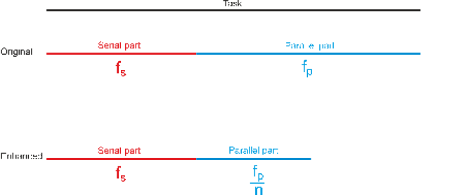
Now, suppose we enhance the performance of a computer by dividing the parallel part into n streams, one per processor, and executing the code on all processors simultaneously. The time taken to execute the task is now fs + fp/n. As you can see, only the parallel part of the task has been affected.
In order to calculate the speedup, S, due to the enhancement, we calculate Toriginal/Tenhanced. In this case the speedup is
S = 1/(fs + fp/n)
We can simplify the equation because we know that fs + fp = 1. Note that we can eliminate either fs or fp. to describe speedup in terms of either the serial or the fractional parts. By convention, the serial part is used. Therefore,
S = 1/(fs + fp/n) = 1/(fs + (1-
The equation is normally rearranged and written as:
S = n/(nfs + 1 -
Let’s look at the boundary values of fs = 1 (all serial) and fp = 0 (all parallel).
When fs = 1, the speedup is n/(nfs + 1 -
If fs = 0 and all processing is parallel, the speedup is n/(nfs + 1 -
Of course the maximum increase in speed can’t be achieved because of the overheads necessary to decompose a task into parallel threads, route them to individual processors, and then recombine the results.
Let’s look at a more typical example. Suppose we are able to run 80% of a program
in parallel and we used a quad-
Now let’s look at another example where the fraction of parallel code is the same
but we use two different speedups. In this case we will use a 16-
n/(nfs + 1 -
Increasing the number of processors from 2 to 16 has changed the speedup from 2.5 to 4. Why have we achieved so little? The answer is that adding a lot more processors has done nothing to reduce the time spent in the serial part of the task. Indeed, if we use an infinite number of processors, the speedup becomes
S = n/(nfs + 1 -
Since fs = 0.2, the ultimate speedup is 1/0.2 = 5.
What Does Amdahl Tell US?
Amdahl’s law confirms the old English saying that ‘It’s no use flogging a dead horse’; that is, it is pointless to apply resources to parts of a system whose contribution to overall performance is small. This is summed up by the expression used in many computer textbooks, ‘Make the common case fast’.
Summary
Computer performance is an important component of the computer architecture curriculum because it concerns all levels of computer user; from the end user who wished to buy the best computer for themselves, to the corporate buyer who might have to purchase 10,000 machines for a large organization, to the chip designer who wants to ensure that their next processor is faster than their competitors.
We have looked at ways in which the performance is defined and measured. In particular, we have introduced metrics that are very poor and to be avoided (clock speed and MIPS) and looked at modern benchmarks such as SPEC that are used by professionals.
Today, processors with multiple CPUs are increasingly becoming the norm in computing. We have introduced Amdahl’s law that helps us evaluate the performance of systems where the processors are replicated to execute parts of the code in parallel. We demonstrated that increasing the number of processors is effective only if code can be parallelized.
Sample Questions
- What is computer performance?
- Why is computer performance difficult to define?
- Why is computer performance difficult to measure?
- In what ways have the performance indicators or performance metrics changed over the years?
- Why is clock speed a very poor indication of performance?
- What is the meaning of MIPS when it is used to refer to computer performance?
- Why is MIPS a poor indication of performance generally?
- When would MIPS be a good indicator of performance?
- In the area of computer performance, what is a benchmark?
- What is the difference between kernel, synthetic, and real benchmarks?
- Why is it more difficult to measure the performance of a computer to be used by a friend or relative than a computer to be used by a nuclear scientist?
- What is Amdahl’s law and what does it teach?
- What is the difference between latency and throughput?
- A computer spends half it time performing hard disk operations. The hard disk is replaced by an SSD (solid state drive) that is ten times faster than the conventional hard drive. What is the increase in the performance of the computer?
- Which application is most likely to benefit from using a faster processor: Adobe Photoshop, or surfing the web? Explain your reasoning.
Clock Cycles per Instruction (CPI)
A computer metric that is often included in textbooks on computer architecture is CPI or clock cycles per instruction. This metric gives an indication of the average number of clock cycles it takes to execute each instruction.
It is not used to measure the performance of computers generally (e.g., by those buying computers) but it is used by those studying computer architecture to evaluate different implementations of the same architecture or to compare compilers.
Suppose a computer’s instruction set can be divided into four categories: arithmetic and logical operations (ALU), load from memory, store in memory, and flow control (Branch). The following table gives the number of clock cycles taken by each of these categories of instruction, and the relative frequency of the instruction class in a program.
Class Frequency Cycles per instruction
ALU 55% 1
Load 20% 10
Store 10% 4
Branch 15% 3
We can use this data to calculate the total number of cycles taken by each instruction class by multiplying the relative frequency by the number of cycles per instruction. For example, loads take 10 cycles and are executed in 20% of the program. The relative number of cycles taken by the load is therefore 10 x 20% = 2 cycles. If we add the relative number of cycles for each instruction (in this case 3.40) we get the average number of cycles per instruction for the program being executed.
Class Frequency Cycles per instruction Total cycles Time
ALU 55% 1 1 x 0.55 = 0.55 0.50/3.40 = 14.7%
Load 20% 10 10 x 0.20 = 2.00 2.00/3.40 = 58.8%
Store 10% 4 4 x 0.10 = 0.40 0.40/3.40 = 11.8%
Branch 15% 3 3 x 0.15 = 0.45 0.45/3.40 = 13.2%
Total 100% 3.40 cycles/instruction
The fifth column gives the percentage of time that the corresponding instruction class takes. This value is the relative frequency divided by the average cycles per instruction; for example, the load class takes 58.8% of the time.
These figures are hypothetical – I made them up for the example. However, if you were a computer designer you would be horrified by the disproportionate amount of time take up by load instructions (half the computation time for an instruction that is only 20% of the program).
Factors in CPU Performance
Suppose we say that the time to execute a program is given by:
Texecute = N x CPI x Tclk
where N is the number of instructions, CPI is the average clock cycles per instruction, and Tcyc is the time for a single clock pulse.
We can list the factors that affect each of these elements in the equation.
N (instruction count) CPI Clock rate
Program Yes
Compiler Yes Yes
Architecture (instruction set) Yes Yes
Organization (microarchitecture) Yes Yes
Technology Yes
The instruction count is dependent on the source (high-
Technology (i.e., the physical manufacturing of the chip) determines how fast the chip can operate and therefore determines the highest clock speed. However, the internal organization determines the highest clock speed too because one organization might have fewer gates in series than another – you can’t clock a chip until all internal signals have passed through their circuits.
NOTE that this does not present the whole picture because it does not include the effect of memory speed, I/O transactions, and disk activity.
Moore’s Law and Performance
One of the most famous laws of computer science is Moore’s law. This law is famous for the following reasons:
Virtually everyone in computing knows about it and quotes it freely
It has a fine pedigree from a major player in the computer industry (Charles Moore)
Moore never stated Moore’s law
Moore’s law is not a law!
Several people in the computing industry such as Douglas Engelbart (one of the inventors
of the mouse) and Alan Turin had predicted the growth in computer power. In 1965
Gordon E. Moore, a chip designer and co-
Moore pointed out that the optimum number of components was doubling every 18 months over the period of his measurements (about 1962 to 1970). This represents an exponential growth curve. Moore later changes the period from 18 months to two years.
Moore’s observation was given the status of a law simply by those who quoted it. In general, the spirit of Moore’s law has held for about four to five decades.
Of course, Moore’s law is not a law of physics. It is an observation that has proved to be true for a remarkably long time. Computer technology has continually evolved so that making smaller, faster, transistors on ever larger silicon chips has continued. Moreover, because Moore’s law has been so successful as a predictor, semiconductor manufacturers have been able to design future generations of chips when (at the current time) the appropriate manufacturing technology does not exist.
Because computer performance is related to the number of transistors on a chip and the speed at which a chip operates, the performance of computer chips have also demonstrated an exponential growth over the decades. Consequently, Moore’s law has been extended to computer performance; that is, when many people use Moore’s law, they intend to say that computer performance has been increasing exponentially and will continue to do so.
However, all good things come to an end and so must Moore’s law. Clearly, if the
number of components on a chip is increasing exponentially, there will come a time
when the size of transistors becomes so small that they are smaller than individual
atoms. Equally, an exponential growth in speed would eventually require faster-
For the time being, 2014, Moore’s law still appears to function, although clock speeds have already reached a barrier at about 4 GHz because of the heat generated inside chips clocked at such high speeds. This clock speed limitation has forced manufacturers to find other ways of increasing speed; in particular, by putting multiple processors on the same silicon chip (e.g., Intel’s multicore processors).
Ironically, there is another less well known law at work in the semiconductor industry.
This is Rock’s law (also called Moore’s second law) and it states that the cost of
a semiconductor chip fabrication plant doubles every four years. Although the cost
per component (transistor) is going down, the manufacturing start-
A consequence of rising fabrication costs is likely to be the concentration of manufacturing in relatively few organizations.