Home Up

Home Teaching Glossary ARM Processors Supplements Prof issues About

Rise of the RISC Processor

Since the introduction of the microprocessor in the mid 1970s, there seemed to have been an almost unbroken trend towards more and more complex – you might even say Baroque – computer architectures. Some of these architectures have developed rather like a snowball by adding layer on layer to a central core as it rolls downhill. A reaction against this trend toward ever increasing complexity began at IBM with the experimental 801 architecture  and continued at Berkeley. Patterson and Ditzel at Berkeley were first to coin the term RISC, or reduced instruction set computer, to describe a new class of streamlined computer architectures that reversed previous trends in microcomputer design. Since then, all the major microprocessor manufacturers have launched their own processors based on the principles established at IBM and Berkeley. All processors now incorporate some elements of the RISC philosophy and the pure RISC machine is no longer fashionable.

Origin of RISC

According to popular wisdom RISC architectures are streamlined versions of traditional complex instruction set computers (that have now become known as CISCs to distinguish them from RISCs). This notion is both misleading and dangerous, because it implies that RISC processors are in some way cruder versions of previous architectures. In brief, RISC architectures redeploys to better effect much of the silicon real estate used to implement complex instructions and elaborate addressing modes in conventional microprocessors of the 68K and 8086 generation. We shall discover that, as several writers have proposed, the term RISC should really stand for regular, or even rationalized, instruction set computer.

If we consider the historical progression of microcomputer architectures as they went from 8-bit to 16-bit to RISC machines, one trend that stands out most clearly is the way in which each new architecture was designed. It’s true, at least to a first approximation, to say that those who designed 8-bit architectures were striving to put a computer on a chip, rather than to create an optimum computing engine. Designers of 16-bit machines attempted to rationalize 8-bit processors by adding features to improve their performance (e.g., by including new addressing modes and more general-purpose registers). Those who conceived RISC architectures took the design process back to fundamentals both by studying what many computers actually do and by starting from a blank sheet (as opposed to modifying an existing chip à la Intel).

The first investigations into computer architectures that later became known as RISC processors did not originate in the microprocessor industry. John Cocke at IBM is usually given credit for the concept of the RISC computer.  In 1974 IBM was involved in a project to design a complex telephone-switching network that required a real-time response and a very fast processor (for the time). Although the project was terminated in 1975, the design work at IBM had highlighted some of the issues at the heart of high-speed computer design. It was clear that a fast computer should avoid direct arithmetic operations on memory (i.e., no instructions such as ADD R0,memory), have a uniform instruction format , include instruction pipelining (i.e., starting executing a new instruction before the current instruction has been completed), and take account of the problems caused by branch instructions.

If the RISC philosophy is so appealing, why was it not developed much earlier? The short answer to this question is that RISC architectures make sense only in a 32-bit world, because RISC processors rely on long instruction formats to help overcome the effect of the processor-memory bottleneck. In other words, it is the progression from 8-bit and 16-bit architectures to 32-bit architectures that has made the development of RISC architectures almost inevitable.

Instruction Usage

A number of computer scientists working independently over a decade or more in the 1970s carried out extensive research into the way in which computers execute programs. Their studies all demonstrate that the relative frequency with which different classes of instructions are executed is not uniform and that some types of instruction are executed far more often than others.

Counting instruction usage is not as simple as you might think. Two metrics of instruction usage can be employed: static and dynamic. In the former, static instruction frequency, the occurrence of each instruction type in a block of code is measured, whereas in the latter, dynamic instruction frequency, the occurrence of each instruction is counted while the program is running. That is, one metric measures compile-time instruction frequency and the other measures run-time instruction frequency. Consider the following example of a fragment of C code that forms the inner product of two matrixes, X and Y.

void main(void)

{

  char X[10], Y[10];

  int  N = 10;

  char s = 0;

  int  i = 0;

  for (i = 0; i < N; i++)

       s = s + X[i] * Y[i];

}

The output from a non-optimizing C compiler for this code using a 68K CISC compiler is:

* Variable X is at -10(A6)

* Variable Y is at -20(A6)

* Variable N is at -22(A6)

* Variable s is at -23(A6)

* Variable i is at -26(A6)

_main

    LINK A6,#-26

*2 {

*3    char X[10], Y[10];

*4    int N = 10;

    MOVE #10,-22(A6)

*5    char s = 0;

    CLR.B -23(A6)

*6    int i = 0;

    CLR -26(A6)

*7    for (i = 0; i < N; i++)

    BRA L1

L2

*8        s = s + X[i] * Y[i];

    MOVE.B -23(A6),D1

    MOVE -26(A6),D0

    CLR.L D7

    MOVE.B -10(A6,D0.W),D7

    CLR.L D6

    MOVE.B -20(A6,D0.W),D6

    MULS D6,D7

    ADD.B D7,D1

    MOVE.B D1,-23(A6)

*(see line 7)

    ADD  #1,-26(A6)

L1 MOVE -26(A6),D7

    CMP -22(A6),D7

    BLT   L2

*9 }

    UNLK A6

    RTS

As we are discussing instruction usage, you might be interested in seeing the same fragment of code when it’s been hand-assembled (this comparison is not entirely fair).

Assembly language form                       Register transfer language form

      CLR.L  D0        [D0]  0                 {Use D0 as S}

      MOVE   #X,A1     [A1]  X                 {A1 points to X}

      MOVE   #Y,A2     [A2]  Y                 {A2 points to Y}

REPEAT

LOOP   MOVE.B (A1),D1   [D1]  [M([A1])]         {get xi}

      MOVE.B (A2),D2   [D2]  [M([A2])]         {get yi}

      MULS   D2,D1     [D1]  [M([A2])].[D1]    {xi x yi}

      ADD.B  D1,D0     [D0]  [D0] + [D1]       {S:= S + xi x yi}

      ADD    #1,A1     [A1]  [A1] + 1          {inc X pointer}

      ADD    #1,A2     [A2]  [A2] + 1          {inc Y pointer}

      CMP    #X+N,A1   [A1] - (X + N)

       BNE    LOOP      UNTIL all N elements added

The static instruction frequency is determined easily by adding up all instances of each type of instruction in the source code. In order to evaluate the dynamic instruction usage, we must either manually walk through the program counting instructions as they are used, or we must run the program on some system that automatically measures instruction frequency. In the example of the hand-assembled code, the static counts for CLR and MULS are the same (i.e., 1). However, the more important dynamic counts are 1 for CLR and N for MULS. This point is significant because CLR is executed in few clock cycles, whereas the more complex multiply instruction requires many more clock cycles.

There has been considerable debate over whether static and dynamic instruction frequencies are correlated. It is tempting to maintain that “If instruction types are uniformly distributed throughout a sufficiently large program, it does not matter whether they are executed inside or outside a loop.” In other words, some believe that in an infinitely large program the ratio of instruction A to instruction B is the same for both static and dynamic instruction counts. Although measurements of static and dynamic instruction frequencies do not yield identical results, there is sufficient correlation between these measurements to regard either of them as a good pointer to instruction usage.

You can divide instructions into groups in several ways; for example, some include arithmetic and logical operations in the same group and some don’t. However, everyone agrees on certain basic principles such as data movement instructions make up a unique group . The following instruction groups have been compiled by Fairclough, who divided machine-level instructions into eight groups according to type.

1. Data movement
2. Program modification (i.e., branch, call, return)
3. Arithmetic
4. Compare
5. Logical
6. Shift
7. Bit manipulation
8. Input/output and miscellaneous

We could debate the validity of these groupings today. However, what we are attempting to do here is to demonstrate the extreme variation in relative instruction frequency between different groups. Fairclough compiled tables of static instruction frequency for seven machines: 6502, 6800, 9900, 68000, NOVA 1210, IBM 360/370 and the Litton computer. Although these are no longer state-of-the-art machines, the results generated by research such as Fairclough’s was instrumental in changing the way in which instruction sets were designed.

Table 1 provides Fairclough’s results and figure 1 illustrates them in histogram form. The data was compiled by analyzing randomly selected programs of many differing types (including assemblers, interpreters, compilers, monitors, kernels, operating system libraries).

Table 1 Relative instruction frequency expressed as a percent

                      Instruction group

Machine     1     2     3      4     5     6     7     8

6502        40.72 26.24 11.49  3.84  5.85  7.04  3.92  0.90

6800        59.52 26.54  4.35  3.68  4.15  1.33  0.43  0.00

9900        36.71 37.24 10.64  6.77  2.36  2.15  4.09  0.04

68000       43.52 25.13 12.09  9.15  5.03  2.65  2.36  0.07

NOVA 1210   37.74 26.53 14.28 10.15  6.08  2.32  1.44  1.46

IBM 360/370 61.48 16.30 13.14  3.80  1.70  3.58  0.00  0.00

Litton      37.24 43.16  9.23  4.05  2.20  1.41  2.12  0.59

Mean value  45.28 28.73 10.75  5.92  3.91  2.93  2.05  0.44

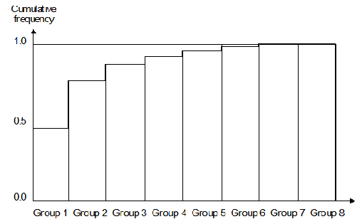
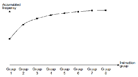
Fairclough fitted a curve, figure 2, to the data in table 1 to obtain the approximate function f(n) = 2-n, where f(n) is the relative frequency of an instruction within group n. Once again, it is necessary to stress the imprecise and empirical nature of these results.

Figure 1 Histogram of relative instruction frequency for seven processors

The data in figure 1 and table 1 convincingly demonstrates that the most common instruction type is the assignment or data movement primitive of the form P = Q in a high-level language or MOVE P,Q or STORE (R1),R0 in a low-level language. Similarly, the program modification group that includes conditional and unconditional branches together with subroutine calls and returns, forms the second most common group of instructions. Taken together, the data movement and program modification groups account for 74% of all instructions. A corollary of this statement is that we can expect a large program to contain only 26% of instructions that are neither data movement nor program modification primitives.

Figure 2 Cumulative relative instruction frequency

An inescapable inference from such results is that processor designers would be better employed devoting their time to optimizing the way in which machines handle instructions in groups one and two, than in seeking new powerful instructions that look impressive in the sales literature. In the early days of the microprocessor, chip manufacturers went out of their way to provide special instructions that were unique to their products. These instructions were then heavily promoted by the company’s sales force. Today, we can see that their efforts should have been directed towards the goal of optimizing the most frequently used instructions (as do today’s chip designers). RISC architectures have been designed to exploit the programming environment indicated by tables 1 and 2. Table 2 provides a summary of the results of various researchers for the relative frequencies (both static and dynamic) of instruction usage. In this table, instruction groups 3 to 7 have been combined into a single column. These figures are even more dramatic than those obtained by Fairclough.

Table 2  A summary of other work on the relative frequency of instruction usage

Authority    Measurement Type         Instruction usage by percent

                                     Group 1 Group 2 Groups 3 - 7

[AlexWort75] static                   48      49      3

[Lunde77]    static                   47      52      1

[Lunde77]    dynamic                  42      56      2

[PatSeq82]   dynamic                  42      54      4

Operand Encoding

It is reasonably true to say that the manufacturers of eight- and 16-bit microprocessors attempted to minimize the size of programs (i.e., create a high code-density) rather than to optimize the performance of their processors. This approach made sense in the late 1970s when memory components were very expensive and there was a great demand for the basic computing power required to implement microcontrollers. In particular, microprocessor designers encoded instructions to yield the smallest possible object code. Due to the byte-oriented nature of early microprocessors, instruction-lengths were chosen as an integer multiple of bytes. Frequently used instructions were given, wherever possible, short instruction lengths (i.e., one byte). Such sophisticated instruction encoding techniques together with variable-length instructions force conventional CISC architectures to adopt very complex instruction decoders. This is a luxury that RISC architectures cannot afford.

By means of careful operand encoding, CISC designers often include frequently used operands as part of the instruction format. For example, a machine-level instruction that increments the contents of a register (i.e., [Register]  [Register] + 1) might be encoded by the short instruction INC Register, rather than the longer form ADD #literal,Register. By taking this approach, the instruction format corresponding to INC register does not require a separate literal field, because the value 1 is implicit in the instruction. This approach to instruction encoding, is similar to the Huffman code sometimes used to compress text.

An obvious question to ask is, “What is the range of the majority of literal operands?” In 1987 Tanenbaum reported that 56% of all constant values lie in the range -15 to +15 and that 98% of all constant values lie in the range -511 to +511. Consequently, the inclusion of a 5-bit constant field in an instruction would cover just over half the occurrences of a literal. RISC architectures have sufficiently long instruction lengths to include a literal field that caters for the majority of all literals.

The importance of data movement primitives and an ability to handle efficiently short literals should be recognized by any designer attempting to implement an optimum architecture. Before we can consider the design of architectures that address themselves to these issues, we still have to consider the nature of operands. It would be very difficult to optimize a data movement primitive if operands were randomly distributed throughout logical address space, because each instruction would have to include an address field spanning all the processor’s address space. We know intuitively that operands are not randomly distributed since the whole basis of cache memory systems relies on the locality of reference.

Measurements made by Tanenbaum, and by Halbert & Kessler indicated that for over 95% of dynamically called procedures just twelve words of storage are sufficient for all their arguments and local values. That is, if an architecture has twelve words of on-chip register storage, it should be able to handle all the operands required by most procedures without accessing main store. Putting these operands in registers both reduces the processor-memory bus traffic and permits small address fields within the instruction format. Moreover, a really efficient architecture should make provision for each procedure to have associated with it about twelve on-chip registers. The transfer of data between registers should be very fast. We shall soon see that some RISC architectures remove the need to transfer data between procedures.

Characteristics of RISC Architectures

We can summarize the previous discussion and lay down a list of the desired characteristics of an efficient RISC architecture.

1. A RISC processor should have sufficient on-chip memory (i.e., registers) to help overcome the worst effects of the processor-memory bottleneck. Internal memory on the CPU chip can be accessed more rapidly than off-chip random access main store. We have stated that procedures require on average less than twelve words for local storage and parameter passing. This fact indicates that it is indeed feasible to adopt on-chip storage.

2. Since instructions in the program modification group that includes procedure call and return instructions are so frequently executed, an effective architecture should make provision for the efficient passing of parameters between procedures.

3. A RISC processor should execute approximately one instruction per clock cycle. CISC architectures sometimes require tens of clock cycles to execute an instruction. Attempting to approach one clock cycle per instruction imposes a limit on the maximum complexity of instructions.

4. RISC architectures should not attempt to implement infrequently used instructions. Complex instructions both waste silicon real estate and conflict with the requirements of point 3 above. Moreover, the inclusion of complex instructions increases the time taken to design, fabricate and test a processor.

5. A corollary of point 3 is that an efficient architecture should not be microprogrammed, as microprogramming interprets an instruction by executing microinstructions. In the limit, a RISC processor itself is close to a microprogrammed architecture in which the distinction between machine cycle and microcycle has vanished.

6. An efficient processor should have a single instruction format (or at least very few formats). By providing a single instruction format, the decoding of an instruction into its component fields can be performed with a minimum level of decoding logic.

7. In order to reduce the time taken to execute an instruction, the multilength instructions associated with first- and second-generation microprocessors should be abandoned. As it would be unreasonable to perform multiple accesses to the program store to read each instruction, it follows that the wordlength of a RISC processor should be sufficient to accommodate the operation code field and one or more operand fields. A corollary of this statement is that a high-speed RISC processor may not necessarily be as efficient as a conventional microprocessor in its utilization of program memory space.

We now look at the three fundamental aspects of the early RISC architectures. First, we describe how it has a large number of on-chip registers and supports a register-to-register architecture. Second, we demonstrate how its use of multiple, overlapping register windows considerably reduces the need to transfer parameters between procedures. Third, we look at its pipelining mechanism that permits the overlapping of instruction execution. Note that windowed-registers is a weak RISC criterion because most of today’s RISC chips do not implement windowing.

Register-based Instruction Sets

Both machine-level and high-level instructions may employ any number of operand fields. The designer of a new architecture must carefully consider the balance between the number of operands per instruction and the way in which an operand is accessed (e.g., from a register or from the main store). Consider the following examples of hypothetical instructions in which V, W, X, Y, Z are operand addresses.

Instruction type Assembly language form RTL form

One operand     CLR X                              [X]   0

Two operands    ADD X,Y                          [Y]   [X] + [Y]

Three operands  ADD X,Y,Z                     [Z]   [X] + [Y]

Four operands    ADD W,X,Y,Z                 [Z]   [W] + [X] + [Y]

Five operands    ADD V,W,X,Y,Z              [Z]   [W] + [X] + [Y] + [Z]

If complexity is no object, there is clearly no limit to the number of fields that might be assigned to an instruction. Research by Tanenbaum  indicates the following frequency of operand sizes:

Single operand:               66%

Double operand:             20%

Three or more operands: 14%

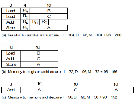
Before we look at the Berkeley RISC’s use of registers, it is instructive to consider a new metric for programs: size. A program contains two components: instructions and data. We can therefore construct a metric that is the sum of a program’s instruction bits plus its data bits. Figure 3, taken from Patterson illustrates how we can calculate the number of bits required to implement the operation A = B + C for three different architectures. In this example we assume that the data words are 32 bits, the address field is 16 bits and the register select field is 4-bits. The three model architectures in figure 3 are: register-to-register, memory-to-register and memory-to-memory. The corresponding metrics for each of these architectures are:

Architecture                  Instruction bits  Data bits     Total bits

Register to register    104                        96                    200

Memory to register     72                         96                   168

Memory to memory    56                         96                   152

These figures appear to indicate that a memory-to-memory architecture offers the best metric and a register-to-register architecture the worst. Serious attention was paid to these metrics in the 1970s, which was a period when main store was relatively expensive and slow, and the large mainframe computer still reigned supreme. The fundamental flaw in metrics like these is that they do not take account of the way in which a large register set can be employed by a compiler. Suppose a compiler is able to allocate register storage to frequently used variables. Once operands have been transferred from main store to working registers, relatively short three-address instructions can be employed to carry out much of the computational work.

Figure 3  Memory requirement as a function of computer architecture (after Patterson)

Now we will discuss the Berkeley RISC I and RISC II architectures. These devices were developed by David Patterson and his colleagues at the university of California in the early 1980s. Although RISC I and RISC II are academic machines constructed to test RISC concepts, they proved to be the prototypes for many later commercial RISC machines. I have called them prototypes because they were to have a greater impact on the computer industry than the IBM 801 project.

The Berkeley RISC I architecture adopts the three-register instruction format specified in figure 4. The 7-bit op-code field defines the nature of the current operation, and a 1-bit SCC field determines whether the condition code is to be updated. The three 5-bit operand fields, source 1, source 2 and destination, each permit one of 25 = 32 internal registers to be accessed. The field marked IM + 8 zeros in figure 4 can used to specify a literal. For our current purposes we are not interested in the SCC and IM+8 zeros fields.

Figure 4  Op-code and operand fields of the RISC I instruction

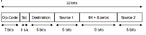
The RISC I instruction format supports dyadic instructions of the form ADD X,Y,Z, where X, Y and Z are internal registers. Since five bits are allocated to each operand field, it follows that the RISC I must have 32 user-selectable internal registers. However, this is emphatically not true, because the Berkeley RISC has 138 user-accessible general-purpose internal registers. The reason for the discrepancy between the number of registers directly addressable by the instruction and the actual number of registers is due to a mechanism called windowing. Windowing, in the context of RISC architectures, provides the programmer with a view of only a subset of all registers at any instant.

An important concept of early RISC processors was the register window, a means of increasing the apparent number of registers. We give this topic its own page.